
Retirement planning – Simulation for the rest of us
A sanity check on our personal retirement savings plans
People knowledgeable about statistics and simulation techniques will find my explanation here overly simplistic, but I think this is an important topic for all of us.
One of the things I’ve come to learn working at Platform Computing and subsequently IBM, is that when it comes to financial planning, we ignore statistics at our peril. There is a reason that investment banks and hedge funds spend millions in the area of risk analytics.
When most of us think about calculating the future value of our retirement savings we do simple math. We take our present savings, assume a rate of return discounted for inflation, factor planned future contributions, consider the number of years that investments and future contributions have to compound, and assume that the result of this calculation represents what we will have in retirement.
The problem with this treatment is that it results in the wrong answer from a statistical point of view. The future value of a portfolio depends not only on the average rate-of-return, but it is also influenced by market volatility and the sequence of returns.
For example, consider that we have $10,000 in the bank and we average a 5% rate of return over three years. There are multiple scenarios that yield an average 5% rate of return, but the actual rates and the order in which they occur turn out to be important in terms of future value (see below). Even in a narrow three year comparison, the divergence in results is considerable. In thirty years, results can be dramatically more divergent. They can make or break retirement plans for a couple or individual.
[table caption=”How the order of returns affects outcomes (average 5% return)” width=”500″ colwidth=”” colalign=””]
Starting principle,Year one(%),End of year one,Year two(%), End of year two, Year three(%), End of Year three
$10000,5%,$10500,5%,$11025,5%,$11576
$10000,-25%,$7500,5%,$7875,35%,$10631
$10000,15%,$11500,5%,$12075,-5%,$11471
[/table]
Calculating the future value of assets is tough, and when it comes to complex systems, simulation is the way to go. The Monte Carlo method is a technique devised shortly after World War II by Stanislaw Ulam who was working at the US Los Alamos National Labs doing nuclear weapons research. The idea is that some systems are sufficiently complex as to defy deterministic solutions. Sometimes the best approach to solving a complex problem is to “simulate outcomes”. We involve reasonable random inputs as factors and evaluate the range of potential outcomes. Building a mathematical model to do this is often possible even in cases where a generalized mathematical solution is not.
In the 1940s modern computer systems did not exist, but even then it was understood that computers were on the horizon and that computer simulation (playing “dice” with random inputs) could be a valuable technique in solving otherwise unsolvable problems. Today Monte Carlo simulation and Stochastic Analysis are staple techniques in fields like engineering and financial risk to model outcomes of real-world behaviors of complex systems.
So what does all this have to do with retirements savings you ask?
When estimating a retirement nest-egg, an average rate of return is not all that useful as the table above shows. Accumulated wealth depends not only on average rates of return, but the sequence of year over year returns and market volatility. It turns out that there is no right answer as to the future value of our retirement portfolios, but computer simulation can at least give us a more accurate picture of the range of future values that are likely given our own personal situations.
Monte Carlo simulation is about letting the computer do the work. In this spirit, I’ve put together an easy-to-use Excel spreadsheet that can help you get started with Monte-carlo simulation in your own financial planning analysis.
Please download a zipped version the Asset Appreciation Model spreadsheet here if you are interested. I think this could be ten minutes well invested.
(Please understand though that any results are worth precisely what you paid for them)
How to use the spreadsheet
Section 1 – Enter your own assumptions here including any retirement savings you might have, estimated rates of return adjusted for inflation as well as a measure of volatility. To explain the volatility measure, if you enter a value of “N” this means that returns could fluctuate by plus or minus N%. For example if our estimate rate of return was “3” and out volatility was “10” we would expect annual returns to fluctuate between -7% and 13%.
Section 2 is calculated for you. This is where the random / stochastic effects come into play. This spreadsheet model will calculate 50 different scenarios given the assumptions you have provided in Section 1 – nothing to see here basically – move on to section 3!
In Section 3 of the spreadsheet, you will see the calculated value of your savings for each scenario given your various assumptions in section 1. This should help you get a picture of the range of possible outcomes at any given year in future.
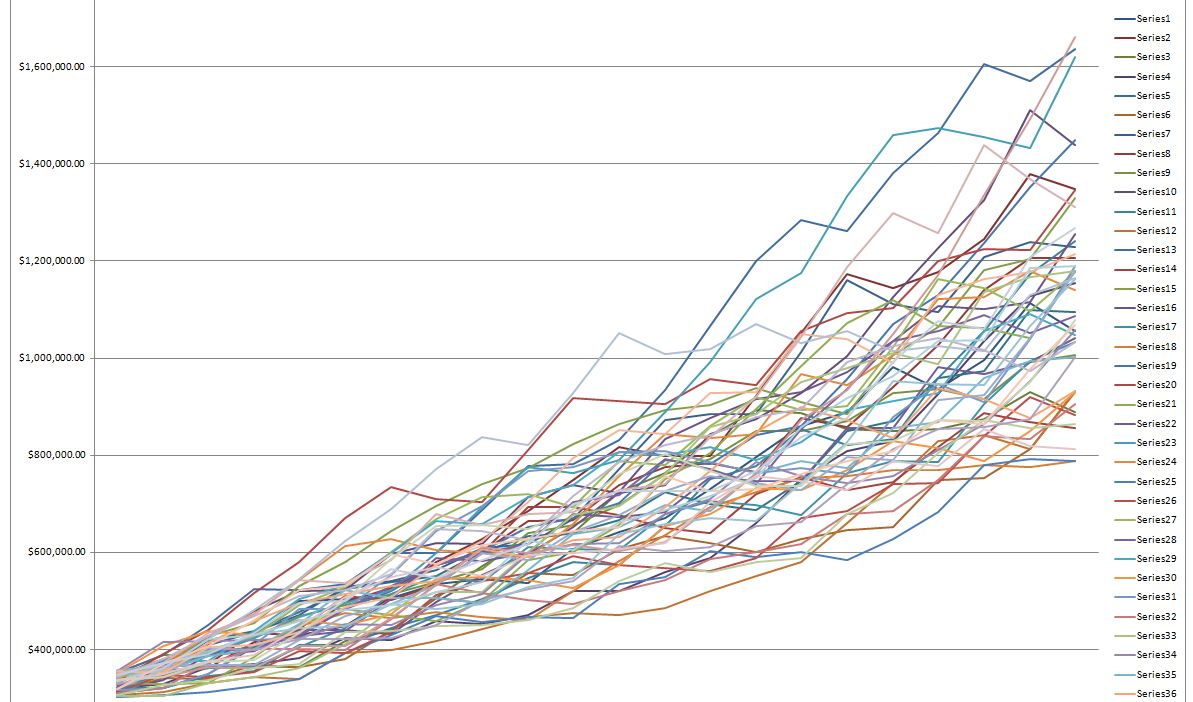
Section 4 puts all this in graphical form, plotting the results of section given a set of assumptions. The figure below shows how given an initial set of assumptions results can diverge. What is useful is that the simulation give you a good sense of the range of possible outcomes. Notice that outcomes are more densely clustered around the mean result. The shape of the outcomes are useful in understanding the risk you face in your personal retirement plan.
Additional notes of explanation
I should mention that every time you do this analysis the results will be different. They will on average cluster around the mean however, so this kind of analysis should offer a reasonable estimate of the risks that you face. I appreciate that this type of analysis is overly simplistic but I think it is useful. Please feel free to modify the spreadsheet supplied as you see fit (and please share your improvements with me? – gord@sissons.ca)
Also – I’m hardly the first person to comment on the importance of this topic and comment on Monte Carlo simulation. Other people have done a better job no doubt devising calculators explaining the issues. Some are free and some are for fee. I wish to make clear that I was very careful to come up with my calculator independently. Others are free to share this and modify as needed without restriction. For a more accurate treatment of the topic please Google “Monte Carlo Retirement Planners” and choose from among many commercial solutions in this area.
Thanks – welcome your views!